Chapter 21. Model Diagnostics and Empirical Credibility

A practical framework for evaluating whether regression results are believable.

Chapter purpose

Estimating a regression model is relatively easy. Determining whether the results are trustworthy is much more difficult.

Applied economists rarely accept regression output at face value. Instead, they examine assumptions, evaluate model fit, inspect residuals, test alternative specifications, and assess whether the estimated relationships are economically sensible.

This process is known as model diagnostics.

In this chapter, we bring together many of the ideas introduced throughout the course and learn how economists evaluate the credibility of empirical results.

Applied question

Can we trust the estimated relationship between fertilizer use and crop yield?

Suppose a researcher estimates the following model:

[ Yield_i = _0 + _1 Fertilizer_i + u_i ]

The coefficient on fertilizer is positive and statistically significant.

Does this automatically mean the result is credible?

Not necessarily.

Before drawing conclusions, we should evaluate the quality of the model.

Economic background

Empirical research is not simply about obtaining significant coefficients.

Researchers must consider questions such as:

  • Is the model correctly specified?
  • Are the assumptions reasonable?
  • Are there unusual observations?
  • Are results sensitive to alternative specifications?
  • Do the estimates make economic sense?

Good empirical work combines statistical evidence with economic reasoning.

Key idea

A useful regression model should satisfy two conditions.

Statistical credibility

The model should be consistent with the assumptions underlying regression analysis.

Economic credibility

The estimated relationships should be sensible from an economic perspective.

A statistically sophisticated model that contradicts basic economic logic is not convincing. Likewise, a theoretically appealing model that fails basic diagnostic checks should be interpreted cautiously.

A diagnostic framework

Whenever you estimate a regression model, ask five questions:

  1. Do the coefficients make economic sense?
  2. Are the coefficients statistically significant?
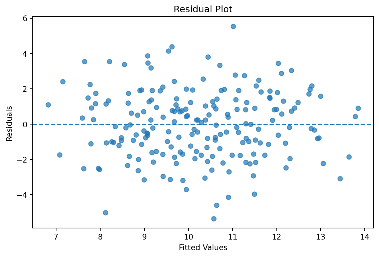
  3. Do the residuals behave reasonably?
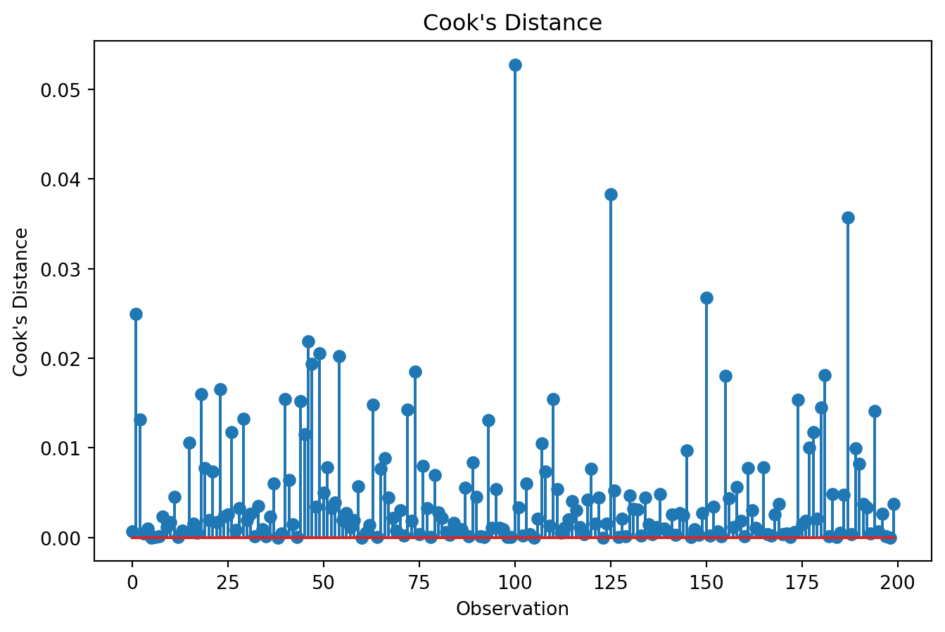
  4. Are there influential observations?
  5. Are the results robust to alternative specifications?

These questions form the foundation of empirical credibility.

Simulating crop yield data

We create a simple dataset to illustrate diagnostic procedures.

import numpy as np
import pandas as pd

np.random.seed(4107)

n = 200

fertilizer = np.random.normal(200, 40, n)

yield_data = (
    2
    + 0.04 * fertilizer
    + np.random.normal(0, 2, n)
)

crop_data = pd.DataFrame({
    "Yield": yield_data,
    "Fertilizer": fertilizer
})

crop_data.head()
Yield Fertilizer
0 10.505050 233.640675
1 11.754481 147.492317
2 12.545903 171.744352
3 8.443709 171.641342
4 11.273924 198.740988

Estimating the model

import statsmodels.api as sm

X = sm.add_constant(
    crop_data["Fertilizer"]
)

y = crop_data["Yield"]

model = sm.OLS(y, X).fit()

print(model.summary())
                            OLS Regression Results                            
==============================================================================
Dep. Variable:                  Yield   R-squared:                       0.378
Model:                            OLS   Adj. R-squared:                  0.374
Method:                 Least Squares   F-statistic:                     120.1
Date:                Thu, 11 Jun 2026   Prob (F-statistic):           3.75e-22
Time:                        06:54:54   Log-Likelihood:                -413.59
No. Observations:                 200   AIC:                             831.2
Df Residuals:                     198   BIC:                             837.8
Df Model:                           1                                         
Covariance Type:            nonrobust                                         
==============================================================================
                 coef    std err          t      P>|t|      [0.025      0.975]
------------------------------------------------------------------------------
const          2.9038      0.682      4.255      0.000       1.558       4.250
Fertilizer     0.0360      0.003     10.960      0.000       0.029       0.042
==============================================================================
Omnibus:                        0.028   Durbin-Watson:                   1.795
Prob(Omnibus):                  0.986   Jarque-Bera (JB):                0.101
Skew:                          -0.025   Prob(JB):                        0.951
Kurtosis:                       2.903   Cond. No.                     1.04e+03
==============================================================================

Notes:
[1] Standard Errors assume that the covariance matrix of the errors is correctly specified.
[2] The condition number is large, 1.04e+03. This might indicate that there are
strong multicollinearity or other numerical problems.

Step 1: Economic plausibility

Before examining diagnostic statistics, consider the coefficient estimates.

Suppose the coefficient on fertilizer equals 0.04.

The interpretation is:

An additional kilogram of fertilizer is associated with approximately 0.04 additional tons of crop yield per hectare.

Questions to consider:

  • Is the sign reasonable?
  • Is the magnitude realistic?
  • Does the result align with agricultural theory?

Economic reasoning should always come before statistical testing.

Step 2: Residual analysis

Residuals reveal information about model performance.

A useful diagnostic plot compares residuals and fitted values.

import matplotlib.pyplot as plt

residuals = model.resid
fitted = model.fittedvalues

plt.figure(figsize=(8, 5))

plt.scatter(
    fitted,
    residuals,
    alpha=0.7
)

plt.axhline(
    y=0,
    linestyle="--"
)

plt.xlabel("Fitted Values")
plt.ylabel("Residuals")
plt.title("Residual Plot")

plt.show()

Interpretation

A good residual plot resembles a random cloud.

Warning signs include:

  • funnel shapes
  • curvature
  • clustering
  • systematic patterns

Such patterns suggest model misspecification.

Step 3: Normality of residuals

Many statistical procedures assume approximately normal residuals.

A Q-Q plot provides a useful visual assessment.

from statsmodels.graphics.gofplots import qqplot

qqplot(
    residuals,
    line="45"
)

plt.title("Q-Q Plot")

plt.show()

Interpretation

If residuals are approximately normal, points should lie close to the 45-degree line.

Moderate deviations are usually acceptable. Large departures may indicate unusual observations or model problems.

Step 4: Model specification

Even if residuals appear reasonable, the model may omit important variables or functional forms.

A common diagnostic is the Ramsey RESET test. The RESET test examines whether additional nonlinear combinations of fitted values improve the model.

Hypotheses

Null hypothesis:

[ H_0: ]

Alternative hypothesis:

[ H_1: ]

Ramsey RESET test

from statsmodels.stats.diagnostic import linear_reset

reset_result = linear_reset(
    model,
    power=2
)

print(reset_result)
<Wald test (chi2): statistic=0.46634025693359565, p-value=0.4946756570547375, df_denom=1>

Interpretation

A small p-value suggests that important information may be missing from the model.

Possible causes include:

  • omitted variables
  • incorrect functional form
  • missing interaction effects
  • nonlinear relationships

Step 5: Influential observations

Some observations exert disproportionate influence on regression results.

These observations deserve careful attention.

Examples include:

  • extremely large farms
  • very unusual households
  • exceptional years
  • recording errors

Influential observations may substantially affect coefficient estimates.

Cook’s Distance

Cook’s Distance measures how much the regression results change when an observation is removed.

from statsmodels.stats.outliers_influence import OLSInfluence

influence = OLSInfluence(model)

cooks = influence.cooks_distance[0]

plt.figure(figsize=(8, 5))

plt.stem(cooks)

plt.title("Cook's Distance")
plt.xlabel("Observation")
plt.ylabel("Cook's Distance")

plt.show()

Interpretation

Most observations should have relatively small influence. A few unusually large values may indicate observations requiring further investigation.

Influential observations are not necessarily incorrect. However, they should always be examined carefully.

Step 6: Robustness checks

Credible research rarely depends on a single specification. Researchers often estimate alternative models.

Examples include:

Alternative variables

Replace one measure with another.

Alternative functional forms

Compare linear, log-linear, and log-log models.

Alternative samples

Estimate the model using the full sample, subsamples, or different time periods.

Alternative standard errors

Compare conventional OLS, robust standard errors, and Newey-West standard errors.

Results that remain stable across alternative specifications are generally more convincing.

Statistical significance versus economic significance

A statistically significant coefficient is not necessarily important.

Example 1

A coefficient implies a 0.001 percent increase in yield. The result is statistically significant, but the economic impact is trivial.

Example 2

A coefficient implies a 15 percent increase in yield. The result is economically important.

Researchers should evaluate both dimensions.

A practical credibility checklist

Before reporting regression results, ask:

Economic logic

  • Do the signs make sense?
  • Are magnitudes reasonable?

Statistical evidence

  • Are coefficients significant?
  • Are confidence intervals reasonable?

Diagnostics

  • Do residuals appear random?
  • Is heteroskedasticity present?
  • Is autocorrelation present?

Model specification

  • Are important variables omitted?
  • Is the functional form appropriate?

Robustness

  • Do results survive alternative specifications?

If several answers are negative, conclusions should be interpreted cautiously.

TipGood empirical habit

Treat diagnostics as evidence, not as a checklist. A model is more credible when its results are statistically defensible, economically sensible, and robust to reasonable alternatives.

Common mistakes

Mistake 1: Focusing only on p-values

Significance alone does not establish credibility.

Mistake 2: Ignoring residuals

Residual analysis often reveals important model weaknesses.

Mistake 3: Assuming diagnostics are formalities

Diagnostics provide valuable information about model quality.

Mistake 4: Ignoring influential observations

A small number of observations can sometimes drive results.

Mistake 5: Confusing statistical significance with economic importance

The two concepts are related but distinct.

Key takeaways

  • Model diagnostics help evaluate empirical credibility.
  • Economic reasoning and statistical evidence should complement one another.
  • Residual plots reveal important information about model performance.
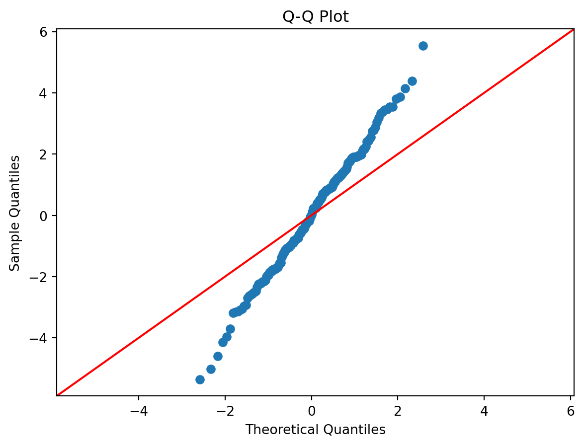
  • Q-Q plots help assess residual normality.
  • The Ramsey RESET test can identify possible misspecification.
  • Influential observations should be examined carefully.
  • Robustness checks strengthen empirical conclusions.
  • Credible research requires more than statistically significant coefficients.

Looking ahead

This chapter concludes Part IV by showing how economists evaluate empirical credibility. In Part V, we shift our focus from explanation to prediction. We explore machine learning methods that are designed to maximize predictive accuracy, often sacrificing some of the interpretability emphasized in traditional econometric models.