Understanding highly correlated regressors, inflated standard errors, and variance inflation factors.
Chapter purpose
Multiple regression allows economists to study the relationship between a dependent variable and several explanatory variables simultaneously. However, problems arise when explanatory variables contain very similar information.
When two or more explanatory variables move together closely, it becomes difficult for the regression model to determine their separate effects. This problem is known as multicollinearity.
In this chapter, we learn what multicollinearity is, how to identify it, and how it affects regression results.
Applied question
Which farm inputs increase crop yield?
Suppose we collect data from 250 farms. Variables include:
crop yield
fertilizer use
irrigation water
farm expenditure
Economic theory suggests that all three inputs contribute to crop productivity. However, farms that spend more money often purchase more fertilizer and use more irrigation. As a result, the explanatory variables may become highly correlated.
Economic background
In real-world datasets, explanatory variables often move together.
Examples include:
education and work experience
income and wealth
farm size and machinery ownership
fertilizer use and irrigation
GDP and energy consumption
When explanatory variables contain overlapping information, the regression model struggles to distinguish their individual contributions.
Multicollinearity is therefore a data problem rather than a modeling mistake.
Key idea
Multicollinearity occurs when explanatory variables are highly correlated.
For example:
[ Corr(X_1,X_2) ]
or
[ Corr(X_1,X_2) ]
In such situations, the regression model receives nearly the same information from multiple variables.
The model can still predict the dependent variable accurately, but coefficient estimates become unstable and difficult to interpret.
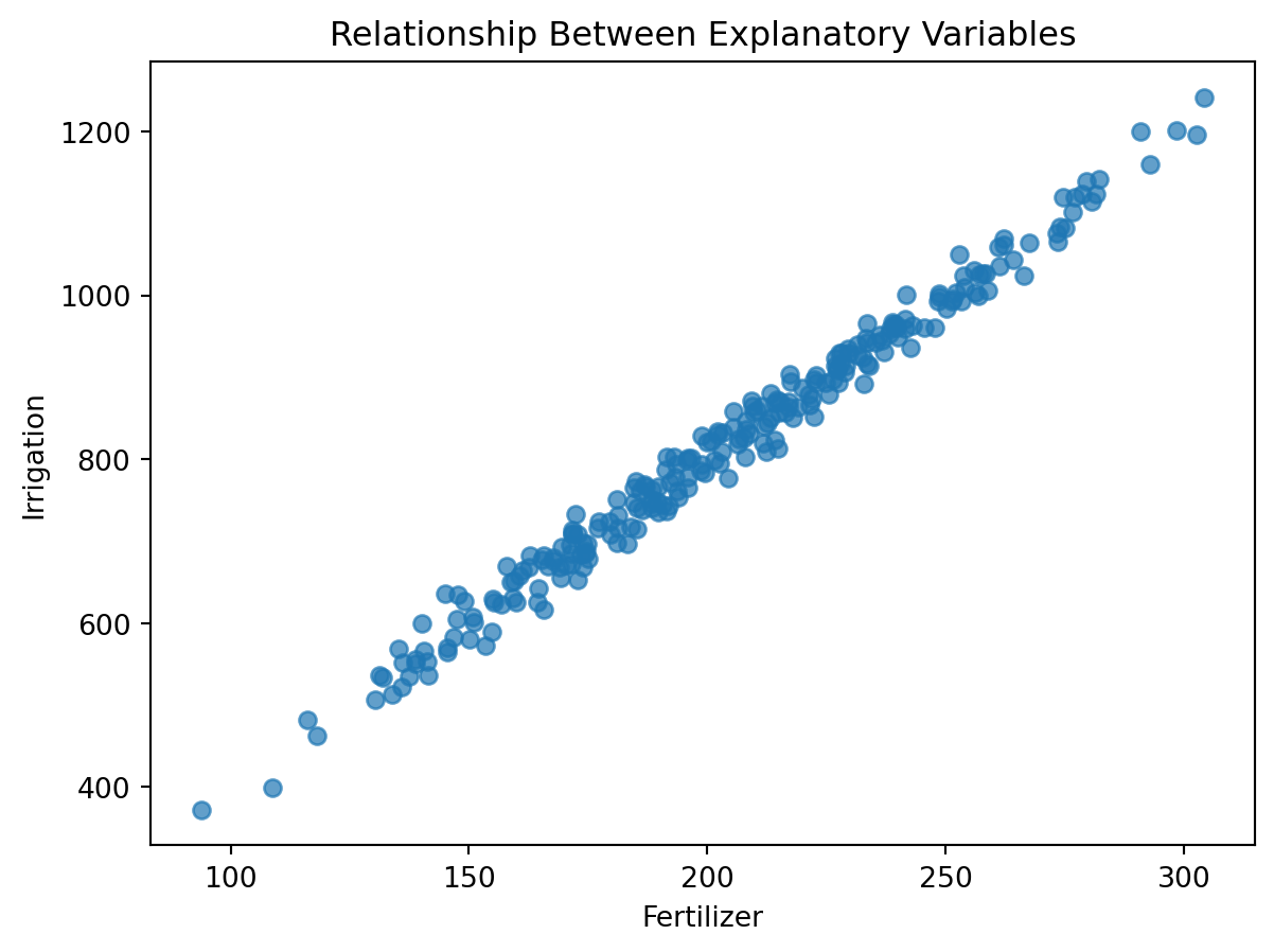
Simulating farm data
To illustrate multicollinearity, we create a dataset in which fertilizer use and irrigation are strongly related.
A common diagnostic tool is the Variance Inflation Factor.
The VIF measures how strongly an explanatory variable can be predicted by the remaining explanatory variables.
VIF
Interpretation
Below 5
Usually acceptable
5 to 10
Potential concern
Above 10
Serious concern
These thresholds are guidelines rather than strict rules.
Calculating VIF
from statsmodels.stats.outliers_influence import variance_inflation_factorvif_data = pd.DataFrame()vif_data["Variable"] = X.columnsvif_data["VIF"] = [ variance_inflation_factor( X.values, i )for i inrange(X.shape[1])]vif_data
Variable
VIF
0
const
25.538392
1
Fertilizer
72.351089
2
Irrigation
72.351089
Interpretation
Large VIF values indicate substantial overlap among explanatory variables.
The larger the VIF, the greater the inflation of coefficient uncertainty.
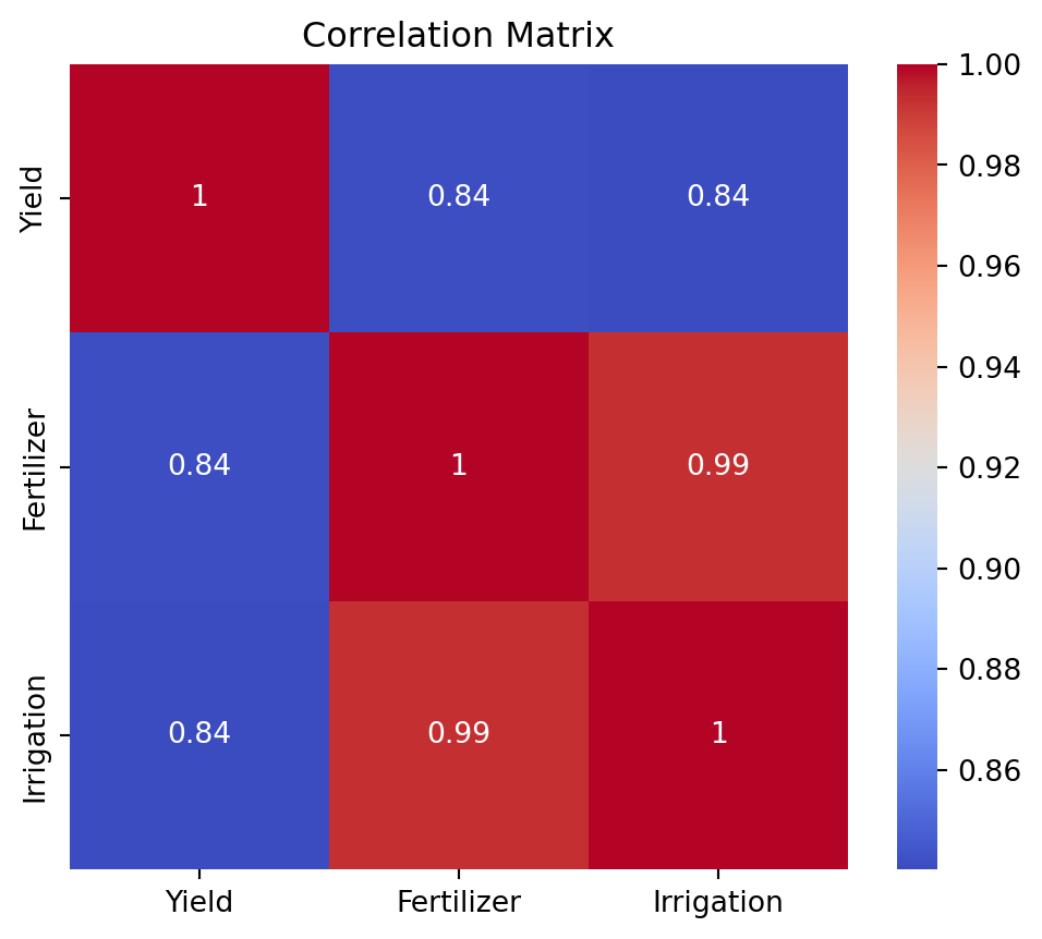
Correlation heatmap
When working with many explanatory variables, a heatmap can provide a useful overview.
import seaborn as snsplt.figure(figsize=(6, 5))sns.heatmap( farm_data.corr(), annot=True, cmap="coolwarm")plt.title("Correlation Matrix")plt.show()
Interpretation
Heatmaps quickly identify highly related variables. However, correlation alone does not fully diagnose multicollinearity because several variables may jointly create the problem.
VIF measures provide a more complete assessment.
Why multicollinearity does not create bias
One of the most common misconceptions is that multicollinearity biases regression coefficients.
This is not generally true.
Multicollinearity primarily affects precision rather than accuracy. The model still estimates the correct relationship on average, but uncertainty increases substantially.
Consequently, coefficient estimates become less reliable.
What can economists do?
Possible responses include:
Collect more data
Additional observations often improve precision.
Remove redundant variables
If two variables measure nearly the same concept, one may be omitted.
Combine variables
Closely related variables can sometimes be merged into an index.
Use economic theory
Theory should guide variable selection. Researchers should not remove variables solely because VIF values appear large.
WarningCommon mistake
Do not drop variables automatically because the VIF is high. Variable selection should be guided by economics, not diagnostics alone.
Common mistakes
Mistake 1: Looking only at (R^2)
A high (R^2) does not guarantee reliable coefficient estimates.
Mistake 2: Treating correlation as proof
High correlation suggests multicollinearity but does not prove it.
Mistake 3: Dropping variables automatically
Variables should not be removed solely because VIF exceeds an arbitrary threshold.
Mistake 4: Confusing bias with imprecision
Multicollinearity usually increases variance rather than creating bias.
Mistake 5: Ignoring economic theory
Variable selection should be guided by economics, not diagnostics alone.
Key takeaways
Multicollinearity occurs when explanatory variables contain overlapping information.
Highly correlated explanatory variables are difficult to separate statistically.
Multicollinearity increases standard errors.
Coefficients may become unstable and insignificant.
Prediction may remain strong even when interpretation becomes difficult.
Variance Inflation Factors provide a useful diagnostic tool.
Multicollinearity generally affects precision rather than bias.
Economic theory remains essential when choosing explanatory variables.
Looking ahead
Multicollinearity makes it difficult to isolate the separate effects of explanatory variables. In the next chapter, we examine endogeneity, which can produce biased coefficient estimates and threaten causal interpretation.