Detecting serially correlated errors and correcting inference using Newey-West standard errors.
Chapter purpose
Many economic datasets are collected over time. Examples include food prices, exchange rates, inflation, GDP, and stock prices. Unlike cross-sectional observations, time-series observations often exhibit persistence. What happens today is frequently related to what happened yesterday.
Regression analysis assumes that error terms are independent from one observation to the next. When this assumption is violated, the model suffers from autocorrelation.
In this chapter, we learn what autocorrelation is, why it occurs, how to detect it, and how to improve inference using Newey-West standard errors.
Applied question
Can monthly wheat prices be explained by a long-term trend?
Suppose we observe monthly wheat prices over several years.
Economic theory suggests that prices may gradually increase over time because of inflation, population growth, and rising production costs.
However, unexpected shocks rarely disappear immediately. If prices are unusually high this month, they may remain above average next month. This persistence often creates autocorrelation.
Economic background
Many economic variables exhibit momentum.
Examples include:
food prices
housing prices
exchange rates
inflation
agricultural commodity prices
A drought that increases wheat prices today may continue affecting prices for several months. Similarly, a recession that reduces consumer demand today may continue influencing economic activity next quarter.
As a result, regression errors often display patterns over time.
Key idea
The classical regression model assumes:
[ Cov(u_t,u_s)=0 ]
for all (t s).
This means that errors from different time periods are unrelated.
Autocorrelation occurs when errors are correlated across time:
[ Cov(u_t,u_{t-1}) ]
Positive autocorrelation is most common. In this case, positive errors tend to be followed by positive errors and negative errors tend to be followed by negative errors.
Simulating wheat price data
To illustrate autocorrelation, we create a synthetic monthly wheat price series. The price follows a trend, while shocks persist through time.
import numpy as npimport pandas as pdnp.random.seed(4107)n =120time = np.arange(n)errors = np.zeros(n)for t inrange(1, n): errors[t] =0.8* errors[t -1] + np.random.normal(0, 5)price =200+0.5* time + errorswheat_data = pd.DataFrame({"Month": time,"Price": price})wheat_data.head()
Month
Price
0
0
200.000000
1
1
204.705084
2
2
197.800607
3
3
195.408530
4
4
193.581992
Visualizing the data
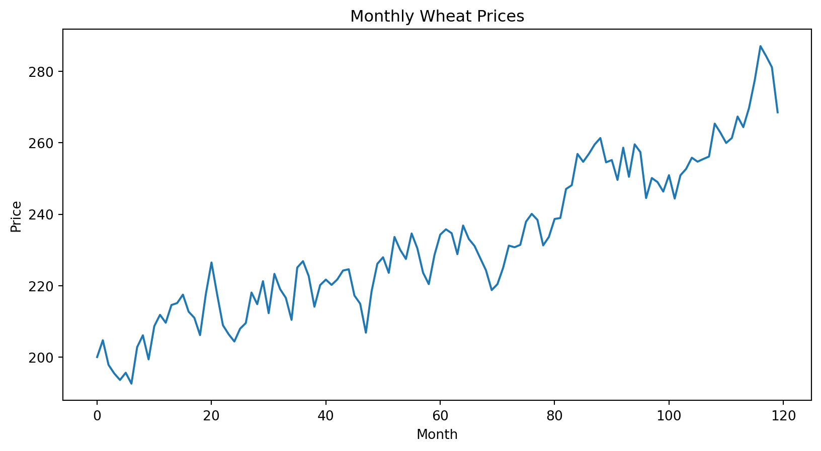
import matplotlib.pyplot as pltplt.figure(figsize=(10, 5))plt.plot( wheat_data["Month"], wheat_data["Price"])plt.xlabel("Month")plt.ylabel("Price")plt.title("Monthly Wheat Prices")plt.show()
Interpretation
The graph shows an upward trend. Notice that prices do not fluctuate randomly around the trend. Instead, periods of high prices tend to cluster together and periods of low prices tend to cluster together.
On average, wheat prices increase by approximately 0.52 units per month.
The coefficient measures the average trend. However, it does not tell us whether the residuals satisfy the assumptions of the regression model.
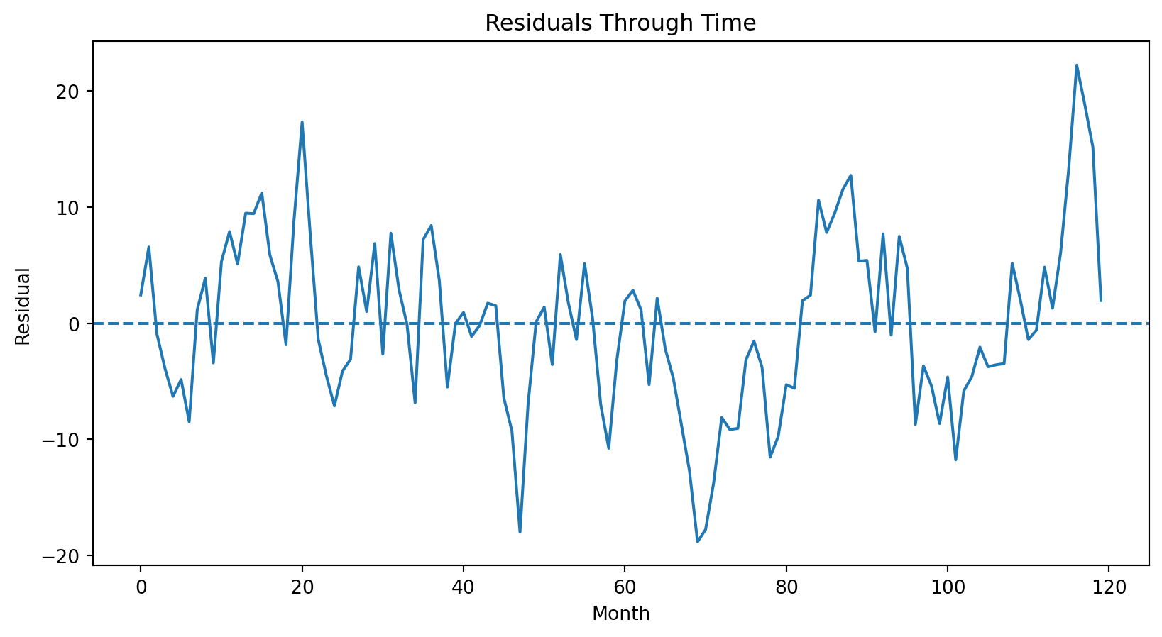
Residual time plot
The first diagnostic is a plot of residuals over time.
residuals = model.residplt.figure(figsize=(10, 5))plt.plot( wheat_data["Month"], residuals)plt.axhline( y=0, linestyle="--")plt.xlabel("Month")plt.ylabel("Residual")plt.title("Residuals Through Time")plt.show()
Interpretation
If residuals are independent, they should bounce randomly above and below zero. Instead, long runs of positive residuals and long runs of negative residuals appear.
This suggests autocorrelation.
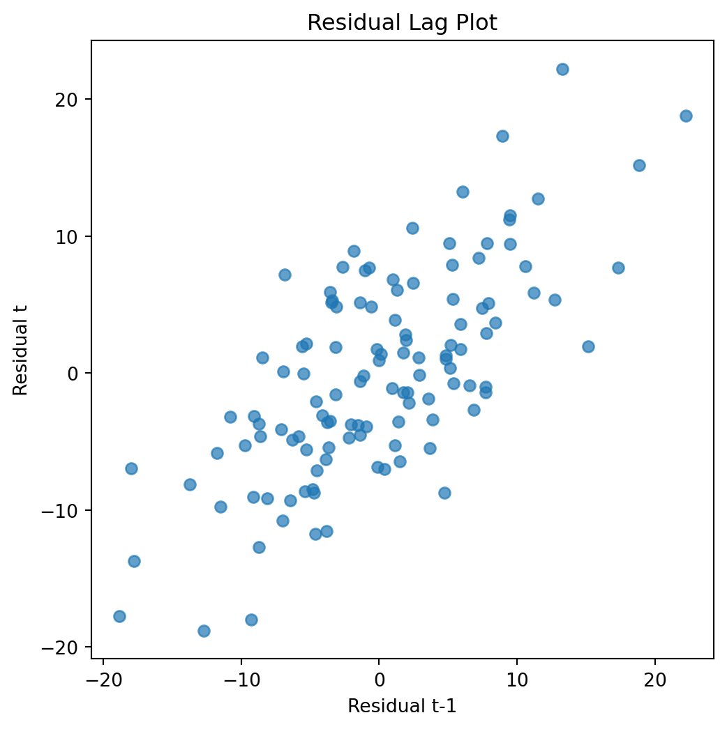
Residual lag plot
Another useful visualization compares each residual with the previous residual.
plt.figure(figsize=(6, 6))plt.scatter( residuals[:-1], residuals[1:], alpha=0.7)plt.xlabel("Residual t-1")plt.ylabel("Residual t")plt.title("Residual Lag Plot")plt.show()
Interpretation
If residuals are independent, the points should form a random cloud. A clear upward pattern indicates positive autocorrelation.
Large positive residuals tend to follow large positive residuals. Large negative residuals tend to follow large negative residuals.
The Durbin-Watson statistic
A commonly used diagnostic is the Durbin-Watson statistic.
from statsmodels.stats.stattools import durbin_watsondw = durbin_watson(model.resid)print(dw)
0.5856399966901465
Interpretation
The Durbin-Watson statistic ranges between 0 and 4.
Value
Interpretation
Around 2
No autocorrelation
Below 2
Positive autocorrelation
Above 2
Negative autocorrelation
In many economic applications, values substantially below 2 indicate positive autocorrelation.
Why autocorrelation matters
Autocorrelation creates several problems. The most important consequence is unreliable standard errors.
This can lead to:
confidence intervals that are too narrow
incorrect hypothesis tests
overstated statistical significance
excessive confidence in results
Just as heteroskedasticity affects inference, autocorrelation primarily affects how we evaluate uncertainty.
Newey-West standard errors
A common solution is to estimate heteroskedasticity and autocorrelation consistent standard errors. These are often called Newey-West standard errors.
                            OLS Regression Results
==============================================================================
Dep. Variable:                  Price   R-squared:                       0.879
Model:                            OLS   Adj. R-squared:                  0.878
Method:                 Least Squares   F-statistic:                     256.5
Date:                Thu, 11 Jun 2026   Prob (F-statistic):           2.25e-31
Time:                        06:54:24   Log-Likelihood:                -411.15
No. Observations:                 120   AIC:                             826.3
Df Residuals:                     118   BIC:                             831.9
Df Model:                           1
Covariance Type:                  HAC
==============================================================================
                 coef    std err          t      P>|t|      [0.025      0.975]
------------------------------------------------------------------------------
const        197.5536      1.993     99.135      0.000     193.607     201.500
Month          0.5801      0.036     16.016      0.000       0.508       0.652
==============================================================================
Omnibus:                        1.304   Durbin-Watson:                   0.586
Prob(Omnibus):                  0.521   Jarque-Bera (JB):                0.839
Skew:                           0.144   Prob(JB):                        0.657
Kurtosis:                       3.291   Cond. No.                         137.
==============================================================================

Notes:
[1] Standard Errors are heteroscedasticity and autocorrelation robust (HAC) using 4 lags and without small sample correction
Comparing standard errors
comparison = pd.DataFrame({"OLS Standard Error": model.bse,"Newey-West Standard Error": nw_model.bse})comparison
OLS Standard Error
Newey-West Standard Error
const
1.361885
1.992766
Month
0.019781
0.036217
Interpretation
The coefficient estimates remain unchanged. Only the estimated uncertainty changes.
Newey-West standard errors generally provide more reliable inference when residuals are correlated over time.
Why time-series data require extra care
Cross-sectional observations are often independent. Time-series observations are rarely independent.
Economic shocks frequently persist. Because of this persistence, economists routinely examine autocorrelation whenever they work with time-series data.
Ignoring autocorrelation can make a model appear more precise than it really is.
WarningCommon mistake
A high (R^2) does not imply independent residuals. A trend model can fit well and still suffer from strong autocorrelation.
Common mistakes
Mistake 1: Ignoring time order
Time-series observations should never be treated as randomly ordered observations. The sequence matters.
Mistake 2: Looking only at (R^2)
A model can have a high (R^2) and still suffer from severe autocorrelation.
Mistake 3: Assuming large samples solve the problem
Autocorrelation can remain important even in very large datasets.
Mistake 4: Reporting conventional standard errors
OLS standard errors may underestimate uncertainty when residuals are correlated.
Mistake 5: Ignoring residual diagnostics
Plots often reveal autocorrelation immediately. Always inspect residual patterns.
Key takeaways
Autocorrelation occurs when regression errors are correlated across time.
Time-series data frequently exhibit persistence.
Residual plots often reveal autocorrelation visually.
The Durbin-Watson statistic provides a useful diagnostic.
Autocorrelation primarily affects standard errors and inference.
Newey-West standard errors often improve reliability.
Economic time series require additional diagnostic checks.
Autocorrelation involves relationships among errors across time. In the next chapter, we examine multicollinearity, which occurs when explanatory variables contain similar information.