milk_data["Volume1000"] = milk_data["Volume"] / 1000Chapter 10. Simple Linear Regression
Chapter Purpose
Economists are often interested in understanding how one variable is related to another. Do larger farms produce more output? Does income increase food expenditure? Do larger milk packages sell for higher prices?
Simple linear regression provides a systematic way to answer such questions.
Using the Milk Data dataset containing 258 milk products, we investigate whether package volume helps explain differences in milk prices.
Applied Question
Do larger milk packages tend to have higher prices?
Volume is defined as:
\[ Volume = Size \times Pieces \]
For easier interpretation, volume is measured in thousands of milliliters:
Exploring the Relationship
sns.scatterplot(data=milk_data, x="Volume1000", y="Price")
plt.title("Milk Price and Package Volume")
plt.xlabel("Volume (1000 ml)")
plt.ylabel("Price")
plt.show()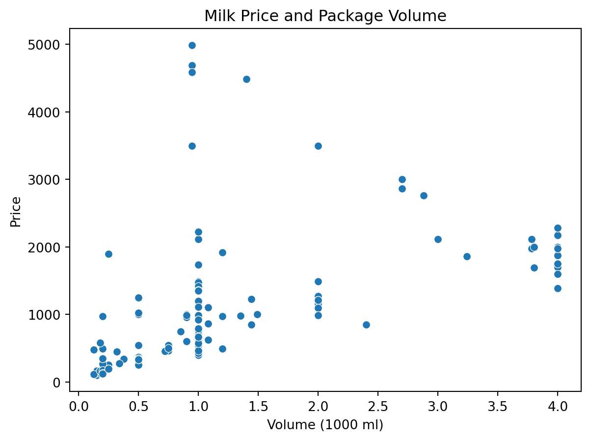
The scatterplot suggests that larger packages generally have higher prices. Regression allows us to quantify this relationship.
The Simple Linear Regression Model
\[ Price_i = \beta_0 + \beta_1 Volume1000_i + u_i \]
where (Price_i) is product price, (Volume1000_i) is package volume in thousands of milliliters, and (u_i) is the error term.
Python Implementation
X = sm.add_constant(milk_data["Volume1000"])
y = milk_data["Price"]
model = sm.OLS(y, X).fit()
print(model.summary())
OLS Regression Results
==============================================================================
Dep. Variable: Price R-squared: 0.274
Model: OLS Adj. R-squared: 0.271
Method: Least Squares F-statistic: 96.56
Date: Thu, 11 Jun 2026 Prob (F-statistic): 1.53e-19
Time: 06:53:02 Log-Likelihood: -2081.5
No. Observations: 258 AIC: 4167.
Df Residuals: 256 BIC: 4174.
Df Model: 1
Covariance Type: nonrobust
==============================================================================
coef std err t P>|t| [0.025 0.975]
------------------------------------------------------------------------------
const 467.9297 74.683 6.266 0.000 320.858 615.002
Volume1000 417.0261 42.439 9.826 0.000 333.451 500.601
==============================================================================
Omnibus: 221.760 Durbin-Watson: 1.652
Prob(Omnibus): 0.000 Jarque-Bera (JB): 2757.298
Skew: 3.610 Prob(JB): 0.00
Kurtosis: 17.295 Cond. No. 3.30
==============================================================================
Notes:
[1] Standard Errors assume that the covariance matrix of the errors is correctly specified.Estimated Regression Model
Using OLS, the estimated equation is:
\[ \widehat{Price} = 516.6 + 417.0 \times Volume1000 \]
based on 258 observations.
Interpreting the Intercept
The intercept is 516.6. This is the predicted price when package volume is zero. Since a package with zero volume does not exist, the intercept has limited economic meaning here. Its main role is positioning the regression line.
Interpreting the Slope
The slope coefficient is 417.0.
A 1,000 ml increase in package volume is associated with an average increase of approximately 417 price units.
The relationship is positive. Larger packages tend to have higher prices on average.
Note
Because volume is measured in thousands of milliliters, the coefficient has a practical interpretation.
Goodness of Fit
The model produces:
\[ R^2 = 0.274 \]
Package volume explains approximately 27.4% of the variation in milk prices. The remaining variation is explained by factors not included in this simple model, such as brand, fat content, package type, freshness, and flavor.
Statistical Significance
The volume coefficient is highly statistically significant:
p < 0.001The 95% confidence interval is:
\[ 333.45 \leq \beta_1 \leq 500.60 \]
The interval does not contain zero, which supports a positive relationship between volume and price.
Residuals
No regression model explains every observation perfectly. The residual is:
\[ Residual_i = Actual_i - Predicted_i \]
milk_data["Predicted"] = model.predict(X)
milk_data["Residual"] = milk_data["Price"] - milk_data["Predicted"]
Visualizing the Fitted Regression Line
sns.regplot(data=milk_data, x="Volume1000", y="Price", scatter_kws={"alpha":0.5})
plt.title("OLS Regression Line")
plt.xlabel("Volume (1000 ml)")
plt.ylabel("Price")
plt.show()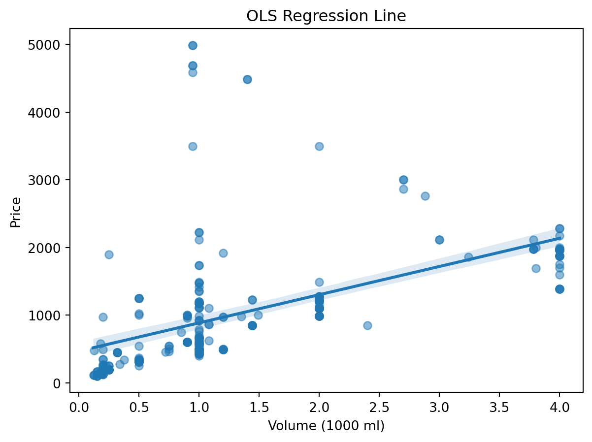
Actual Versus Predicted Values
plt.scatter(milk_data["Price"], milk_data["Predicted"])
plt.xlabel("Actual Price")
plt.ylabel("Predicted Price")
plt.title("Actual vs Predicted Prices")
plt.show()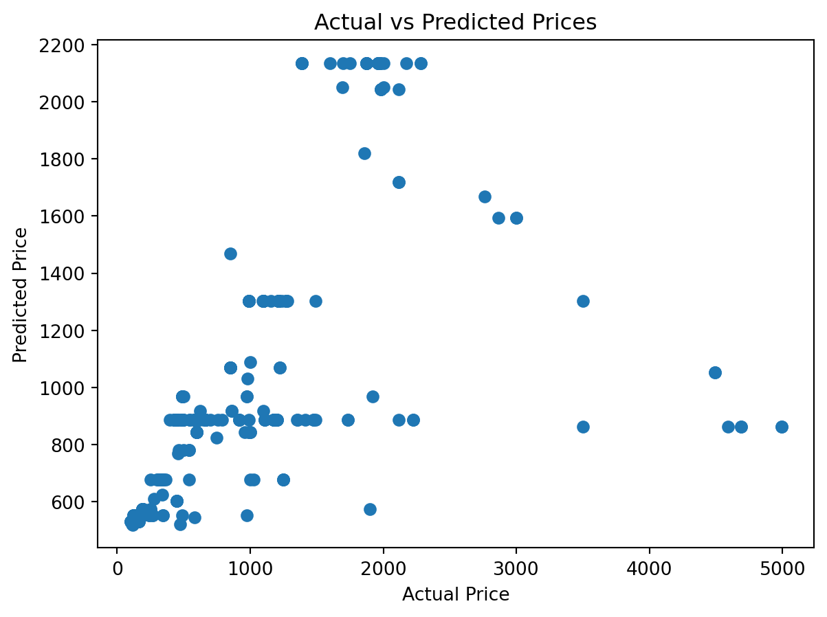
Regression Does Not Prove Causality
The positive coefficient does not necessarily imply that increasing package volume causes price to increase. Premium brands may sell larger products, higher-quality products may come in larger packages, or marketing strategies may differ across package sizes.
Warning
A statistically significant coefficient does not automatically imply a causal effect.
Common Mistakes
WarningCommon Mistake 1
Interpreting association as causation.
WarningCommon Mistake 2
Ignoring the units of measurement.
WarningCommon Mistake 3
Overinterpreting the intercept.
Key Takeaways
- The Milk Data regression uses 258 observations.
- The estimated equation is (=516.6+417.0Volume1000).
- A 1,000 ml increase in volume is associated with an average price increase of about 417 price units.
- The relationship is statistically significant.
- The model explains 27.4% of the variation in milk prices.
- Additional factors motivate multiple regression analysis.