Regression models can be used for prediction, but prediction is useful only when model performance is assessed carefully. This chapter uses the Milk Data model to explain fitted values, residuals, R², MAE, and RMSE.
Package volume explains approximately 27.4% of the variation in milk prices. The remaining 72.6% is explained by other factors not included in this simple model.
model.rsquared
np.float64(0.27387839998291263)
Prediction Accuracy
Using the actual Milk Data regression:
\[
MAE = 437.6
\]
\[
RMSE = 772.0
\]
MAE means that predictions differ from actual prices by about 438 price units on average. RMSE is larger because it penalizes large prediction errors more strongly.
mae = mean_absolute_error(milk_data["Price"], milk_data["Predicted"])rmse = root_mean_squared_error(milk_data["Price"], milk_data["Predicted"])mae, rmse
(437.5678085533861, 772.0000524580844)
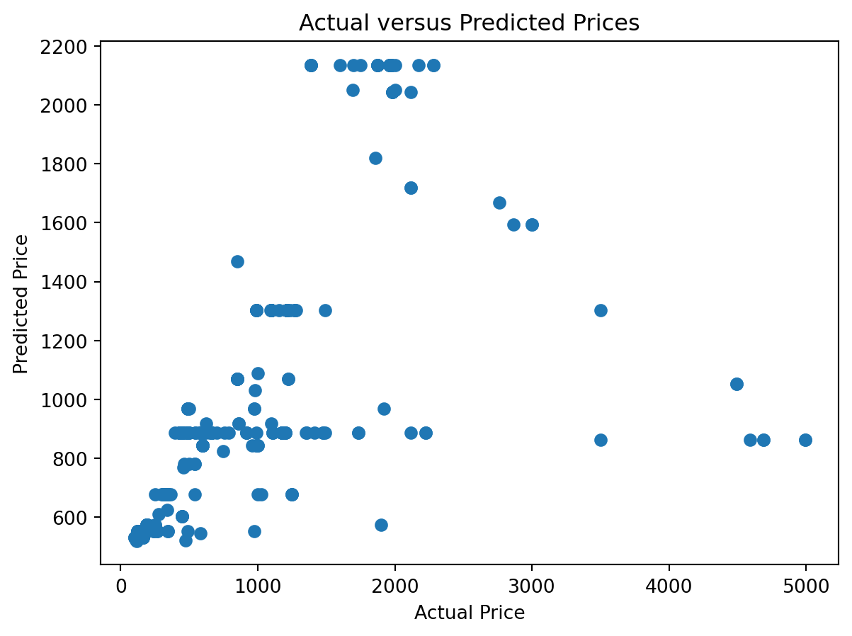
Actual Versus Predicted Plot
plt.scatter(milk_data["Price"], milk_data["Predicted"])plt.xlabel("Actual Price")plt.ylabel("Predicted Price")plt.title("Actual versus Predicted Prices")plt.show()
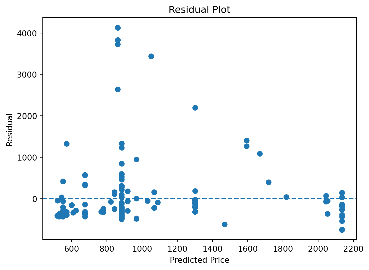
A good residual plot should show random scatter with no systematic pattern.
Prediction Versus Explanation
Prediction and explanation are related but not identical. Prediction focuses on accuracy. Explanation focuses on economic interpretation. A model can predict well without being causal, and a model can be useful for explanation even with modest prediction power.
Warning
A high R² does not prove causality and does not guarantee that the model is correctly specified.
What We Learned From the Milk Data
R² = 0.274
MAE = 437.6
RMSE = 772.0
Volume is useful but not sufficient. Additional variables are needed to improve prediction and explanation.
Key Takeaways
Fitted values are predicted values.
Residuals measure prediction errors.
Volume explains 27.4% of milk price variation.
MAE is approximately 437.6 price units.
RMSE is approximately 772.0 price units.
Prediction and explanation are distinct objectives.