Chapter 17. Heteroskedasticity and Robust Standard Errors
Detecting non-constant error variance and correcting inference using robust standard errors.
Chapter purpose
Regression analysis is one of the most widely used tools in applied economics. However, obtaining coefficient estimates is only the first step. Economists must also determine whether the reported standard errors, confidence intervals, and hypothesis tests are reliable.
One of the most common violations of the classical regression assumptions is heteroskedasticity. Heteroskedasticity occurs when the variability of the regression errors changes across observations. In practice, larger farms, firms, households, or countries often exhibit greater variability than smaller ones.
Ignoring heteroskedasticity can lead to misleading conclusions about statistical significance. In this chapter, we learn how to identify heteroskedasticity, formally test for it, and correct inference using robust standard errors.
Applied question
Do larger farms earn higher income?
Suppose we collect information from 200 farms and estimate the relationship between annual farm income and farm size.
Economic theory suggests that larger farms generally earn higher income. However, larger farms may also face greater uncertainty because they operate on a larger scale and are more exposed to weather shocks, market fluctuations, and production risks.
As a result, income variability may increase with farm size.
Economic background
Many econometric applications involve observations with very different scales.
Examples include:
small and large farms
small and large firms
low-income and high-income households
small and large countries
When the variability of outcomes increases with size, the assumption of constant error variance may be violated.
For example, a small farm may earn between 4,000 and 6,000 OMR annually, while a large farm may earn between 20,000 and 60,000 OMR. The average income increases with farm size, but so does the uncertainty surrounding income.
Key idea
The classical linear regression model assumes that the variance of the error term is constant across all observations:
[ Var(u_i)=^2 ]
This assumption is known as homoskedasticity.
Heteroskedasticity occurs when the error variance changes across observations:
[ Var(u_i)^2 ]
In practical terms, some observations are measured with greater uncertainty than others.
The presence of heteroskedasticity does not necessarily bias the estimated regression coefficients. However, it can make standard errors unreliable, leading to incorrect confidence intervals and hypothesis tests.
Simulating farm data
To illustrate heteroskedasticity, we create a synthetic dataset in which larger farms have both higher income and greater income variability.
import numpy as npimport pandas as pdnp.random.seed(4107)n =200land = np.random.uniform(5, 500, n)error = np.random.normal(0, land *20, n)income =5000+120* land + errorfarm_data = pd.DataFrame({"Income": income,"Land": land})farm_data.head()
Income
Land
0
24672.435314
138.996820
1
45479.198779
325.219332
2
21225.941326
116.010498
3
16007.881758
116.506283
4
11574.007515
58.509175
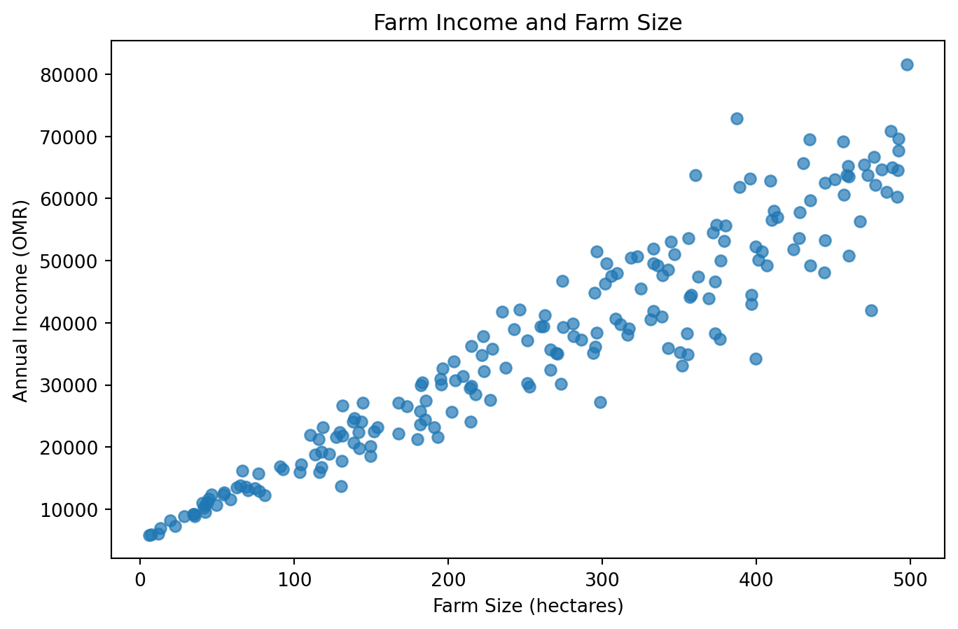
Visualizing the relationship
Before estimating a regression model, it is always useful to inspect the data visually.
import matplotlib.pyplot as pltplt.figure(figsize=(8, 5))plt.scatter( farm_data["Land"], farm_data["Income"], alpha=0.7)plt.xlabel("Farm Size (hectares)")plt.ylabel("Annual Income (OMR)")plt.title("Farm Income and Farm Size")plt.show()
Interpretation
The graph shows a clear positive relationship between farm size and income.
Larger farms tend to earn higher income. However, the spread of observations becomes wider as farm size increases. Small farms cluster relatively closely together, whereas large farms exhibit much greater variation.
This visual pattern suggests heteroskedasticity.
Estimating the regression model
We estimate a simple linear regression model:
[ Income_i = _0 + _1 Land_i + u_i ]
where (Income_i) is annual farm income, (Land_i) is farm size, and (u_i) is the random error term.
                            OLS Regression Results
==============================================================================
Dep. Variable:                 Income   R-squared:                       0.902
Model:                            OLS   Adj. R-squared:                  0.901
Method:                 Least Squares   F-statistic:                     1815.
Date:                Thu, 11 Jun 2026   Prob (F-statistic):          1.14e-101
Time:                        06:54:14   Log-Likelihood:                -2010.0
No. Observations:                 200   AIC:                             4024.
Df Residuals:                     198   BIC:                             4031.
Df Model:                           1
Covariance Type:            nonrobust
==============================================================================
                 coef    std err          t      P>|t|      [0.025      0.975]
------------------------------------------------------------------------------
const       5031.2341    838.222      6.002      0.000    3378.246    6684.222
Land         120.8008      2.835     42.606      0.000     115.210     126.392
==============================================================================
Omnibus:                       15.725   Durbin-Watson:                   1.895
Prob(Omnibus):                  0.000   Jarque-Bera (JB):               39.693
Skew:                          -0.248   Prob(JB):                     2.40e-09
Kurtosis:                       5.125   Cond. No.                         622.
==============================================================================

Notes:
[1] Standard Errors assume that the covariance matrix of the errors is correctly specified.
Interpreting the coefficient
Suppose the estimated slope coefficient equals 118.
The interpretation is:
On average, each additional hectare of land is associated with approximately 118 OMR higher annual farm income.
This interpretation focuses on the average relationship. The regression coefficient does not describe the variability of income around that relationship.
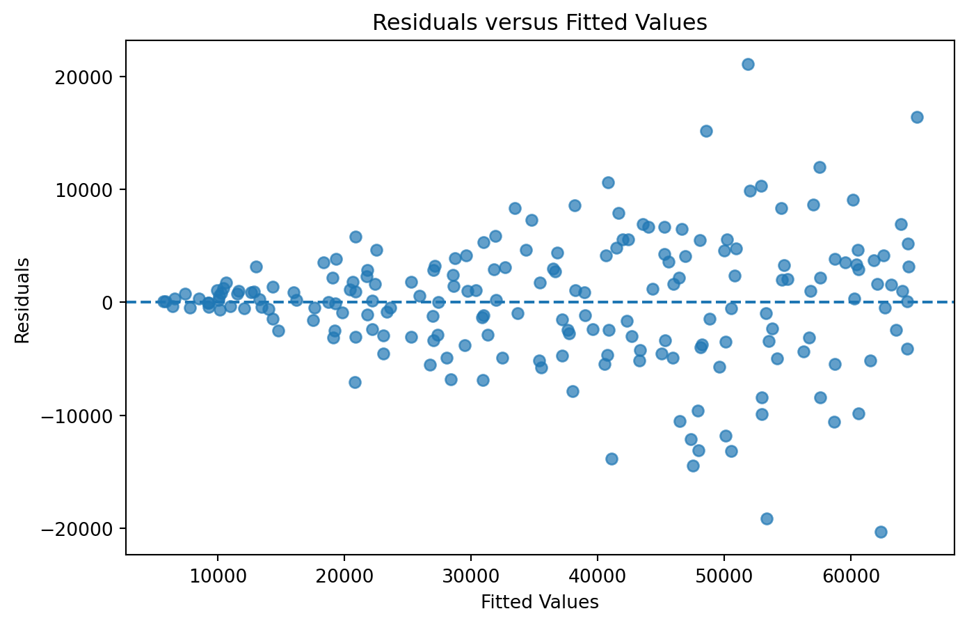
Residual analysis
A residual plot is often the simplest way to detect heteroskedasticity.
If the homoskedasticity assumption holds, the residuals should display a roughly constant vertical spread across all fitted values.
Instead, the residual plot resembles a funnel. Residuals become increasingly dispersed as fitted values increase. This pattern is one of the most common indicators of heteroskedasticity.
The Breusch-Pagan test
Visual inspection is useful, but economists often supplement graphs with formal statistical tests.
The Breusch-Pagan test evaluates whether the variance of the residuals changes systematically across observations.
Hypotheses
Null hypothesis:
[ H_0: ]
Alternative hypothesis:
[ H_1: ]
from statsmodels.stats.diagnostic import het_breuschpaganbp_test = het_breuschpagan( model.resid, model.model.exog)labels = ["LM Statistic","LM p-value","F Statistic","F p-value"]for name, value inzip(labels, bp_test):print(name, value)
LM Statistic 24.852888240654703
LM p-value 6.187626749033513e-07
F Statistic 28.095649549796637
F p-value 3.0665931032837663e-07
Interpretation
A small p-value indicates evidence against the null hypothesis of constant variance.
If the p-value is below 0.05, heteroskedasticity is typically considered statistically significant.
Why heteroskedasticity matters
Many students believe that heteroskedasticity changes coefficient estimates. This is usually incorrect.
The primary problem is that heteroskedasticity affects standard errors.
As a result:
confidence intervals may be inaccurate
hypothesis tests may be misleading
statistically significant results may become insignificant
insignificant results may appear significant
Consequently, economists focus on correcting inference rather than changing coefficient estimates.
Robust standard errors
One of the most common solutions is to estimate robust standard errors.
Robust standard errors adjust the estimated variability of the coefficients without changing the coefficient estimates themselves.
comparison = pd.DataFrame({"OLS Standard Error": model.bse,"Robust Standard Error": robust_model.bse})comparison
OLS Standard Error
Robust Standard Error
const
838.221999
490.888159
Land
2.835285
2.726142
Interpretation
The coefficient estimates remain unchanged because the regression line itself is unchanged. However, the estimated uncertainty surrounding the coefficients may increase or decrease.
The purpose of robust standard errors is to provide more reliable inference when heteroskedasticity is present.
Why robust standard errors are common
Many modern empirical studies routinely report robust standard errors.
Reasons include:
heteroskedasticity is common in economic data
robust standard errors are easy to calculate
they improve the reliability of hypothesis testing
Logarithmic transformations sometimes reduce heteroskedasticity but should not be applied without economic justification.
Mistake 5: Reporting only conventional standard errors
When heteroskedasticity is suspected, robust standard errors are often preferable.
Key takeaways
Heteroskedasticity occurs when error variance is not constant across observations.
Larger economic units often exhibit greater variability than smaller units.
Residual plots provide a useful visual diagnostic.
The Breusch-Pagan test provides a formal statistical test.
Heteroskedasticity mainly affects standard errors and inference.
OLS coefficient estimates often remain unchanged.
Robust standard errors provide more reliable hypothesis tests and confidence intervals.
Careful diagnostics improve the credibility of empirical research.
Looking ahead
Heteroskedasticity involves changing error variance across observations. In the next chapter, we examine a different problem that arises in time-series data: autocorrelation.